

“Over the years we’ve invested significantly in our field data team - focusing on producing trusted ratings. While this ensures the accuracy of our Ratings, it doesn’t allow the scale across the thousands of projects that buyers are considering.”

For more information on carbon credit procurement trends, read our "Key Takeaways for 2025" article. We share five, data-backed tips to improve your procurement strategy.
One more thing: Connect to Supply customers also get access to the rest of Sylvera's tools. That means you can easily see project ratings and evaluate an individual project's strengths, procure quality carbon credits, and even monitor project activity (particularly if you’ve invested at the pre-issuance stage.)
Book a free demo of Sylvera to see our platform's procurement and reporting features in action.
The challenge behind remote sensing data for carbon projects
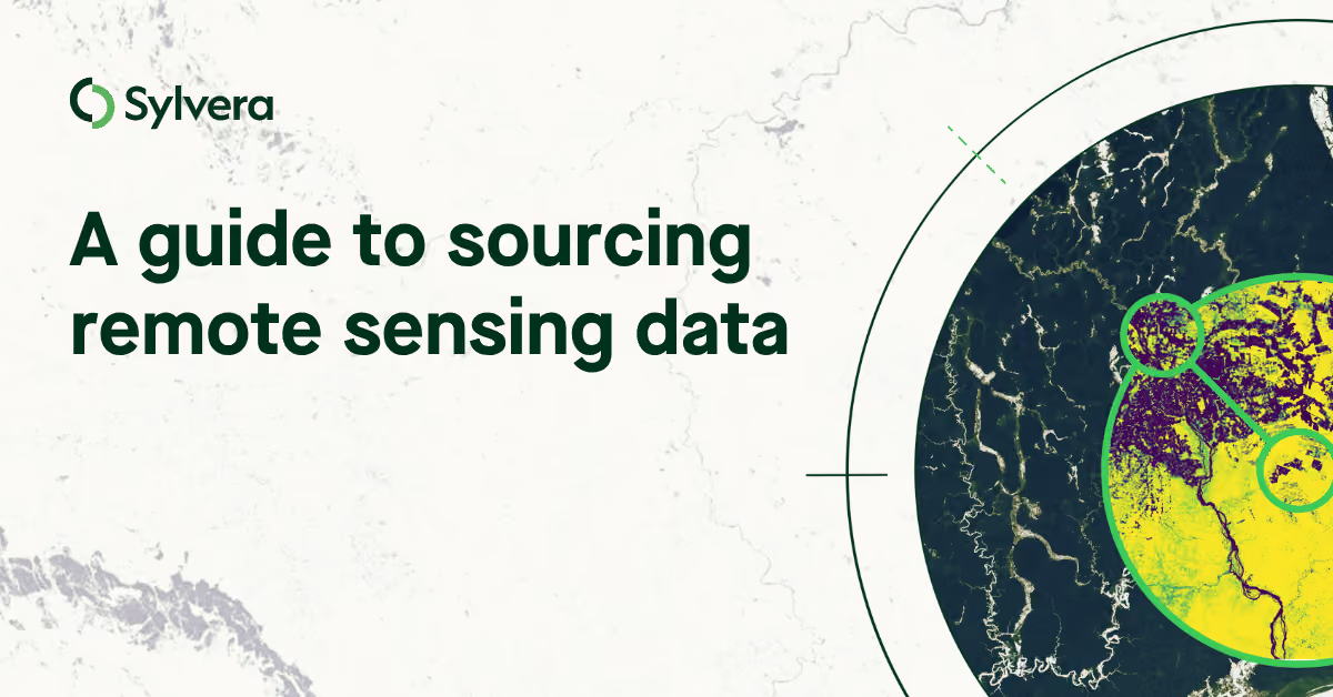
If you're developing an afforestation, reforestation, or revegetation (ARR) project, you’ll now need to source a geospatial dataset. That's especially true for VM0047 projects, where several data service providers are formally vetted by Verra to supply stocking index data. And the requirement is becoming common well beyond VM0047.
In practice, for developers that usually means talking to two or three providers, requesting test data from each, and discovering that their numbers don't fully agree. At that point, the natural move is to compare each provider's pixel data against your own field plots - the trees you or a partner physically measured and ran through an allometric equation - and pick whoever matches best.
The problem is that neither dataset is ground truth. There's no independent measurement of biomass across your entire project area to check either one against.
Field plots are the closest thing to a reference, but they cover a small fraction of the site and carry major uncertainty of their own. So a straight plot-versus-pixel comparison can't fully settle which provider is right.
The pitfalls of a simple plot-to-pixel comparison
There are four reasons a straightforward comparison can mislead you, and none of them mean the data is bad.
The gap isn’t "who's wrong." Field plots run tape measurements through an allometric equation. Pixel data comes from a satellite model. If the two show different average stocks, that gap alone doesn't tell you which one is closer to the truth, they're two different measurement approaches, not a right answer and a wrong one.
Weak correlation isn't weak data. If you plot field values against pixel values, you'll often see a best-fit line that's flatter than the 1:1 line you'd expect from a perfect match. That's usually not a sign of bad data - it's regression dilution, where uncertainty in both the field and pixel measurements (often over 50% on each side) mechanically pulls the correlation down.
Small samples are a coin toss. With 20 plots or fewer, and both sides carrying roughly 50% uncertainty, randomness dominates. Measure a different 20 plots and the ranking can flip. You could easily rank a weaker provider above a stronger one and never know it.
A plot can land in the wrong pixel. GPS typically locates a plot to within 5–15 meters, but pixels are only 10–30 meters across. A plot can fall in a neighboring pixel, or straddle several. That's a scale-and-location mismatch, not a flaw in either dataset.
Compared this way, the winner often comes down to randomness rather than merit - which is a real risk if you're trying to make a defensible sourcing decision.
Getting more out of the field data you have
None of this means field plots shouldn’t be used for comparison. It means point-by-point matching is the wrong way to use them. Three adjustments make the comparison far more reliable.
Match plots to pixels properly. Use as many plots as you have, and larger ones where possible. CEOS good practice recommends at least around 0.25 hectares, which cuts down noise and scale mismatch. Buffer each plot by a conservative geolocation error (roughly 10–20 meters), then match it to the best-fitting pixel within that buffer, not simply the nearest one.
Compare stratum means, not individual points. Group plots and pixels into strata - forest type is a common one - and compare the average of each stratum rather than matching plot by plot. Random noise tends to average out at this level, so a real difference between providers becomes visible where individual points can't show it. This only works if your plots represent each stratum, rather than being clustered wherever access was easiest.
Compare distributions. Plot the remote sensing data's distribution across the wider stratum and overlay your field plots on it. The question becomes whether your plots fall within that range, not whether each one matches its exact pixel. Again, this depends on your plots spanning the site's strata and biomass range, not just the convenient parts of it.
When field plots aren't enough: airborne lidar
If you have access to it, airborne (or even low-cost drone) lidar gives a stronger reference than field plots alone. It provides thousands of validation pixels across tens or hundreds of hectares rather than a handful of plots, which is enough coverage that the randomness affecting small samples largely disappears.
Because lidar assigns a value to every pixel, you're comparing like with like at matching scale, so the geolocation mismatch that undermines plot-to-pixel comparisons goes away.
It also lets you validate more than aboveground biomass. Canopy height and canopy cover come almost directly from lidar, so those layers can be checked cleanly; biomass still requires a structure-to-biomass model layered on top, so it remains one step less direct.
And drone lidar has made this kind of reference achievable without the budget that a full airborne campaign once required.
Choosing well, with or without field data
If you have field data, use it the right way. Match plots to pixels within a geolocation buffer, compare stratum means rather than individual points, and compare distributions rather than single matches. Avoid raw point-to-pixel comparison as it's the version most likely to reward chance over quality.
Alongside your field data, judge the provider directly on two things:
Requirements - does the data fit what you need? Resolution, update cadence, and the specific layers (biomass, canopy structure, indices) your methodology requires.
Trust - how is the data validated? What was the underlying model trained on, has it been independently validated against a reference, and does it hold up specifically in your area of interest?
The goal is to choose on merit rather than on a comparison too noisy to settle the question:
Whether the data fits
Whether you can trust it
Whether it's representative of your project area
That's how you avoid rejecting good data, or ending up with weaker data, by chance.
Get a quick-reference downloadable version of this guide here [Download the PDF version here].
Where Sylvera fits into this
The guidance above holds regardless of which provider you're evaluating. If you're weighing Sylvera's Biomass Atlas as one of your options, here's what it's worth knowing around the points raised above.
Biomass Atlas provides aboveground biomass and canopy height globally, at 10 to 30 meter resolution, with annual coverage from 2000 to the present, delivered via API.
On the trust side: it's calibrated against more than 250,000 hectares of proprietary multi-scale lidar collected across diverse ecosystems, and validated to within ±3% of field-based destructive measurements. Sylvera is also one of the small number of data service providers Verra has vetted to supply stocking index data for VM0047 — which speaks to how the data is produced, though it doesn't substitute for the representativeness checks this guide covers, since those still depend on your specific project area.
Where the data gets applied to a specific methodology's requirements such as applicability screening, donor pool construction, dynamic baselines, and performance benchmarking, Sylvera's Methodology Toolkit comes in. It's built on top of Biomass Atlas, so the same underlying data supports both self-serve access to the raw data and a fully managed analysis, depending on what your team needs.